Data Structures and Algorithms (Adjacency Lists and Adjacency Matrix) - Tirthankar Pal - MBA from IIT Kharagpur, GATE, GMAT, IIT Written Test, Interview were a part of MBA Entrance, B.S. in Computer Science from NIELIT

A graph can be represented using 2 data structures- adjacency matrix and adjacency list

An adjacency matrix can be thought of as a table with rows and columns. The row labels and column labels represent the nodes of a graph. An adjacency matrix is a square matrix where the number of rows, columns and nodes are the same. Each cell of the matrix represents an edge or the relationship between two given nodes. For example, adjacency matrix Aij represents the number of links from i to j, given two nodes i and j.

For example, adjacency matrix Aij represents the number of links from i to j, given two nodes i and j. 

	A	B	C	D	E
A	0	0	0	0	1
B	0	0	1	0	0
C	0	1	0	0	1
D	1	0	0	1	0
E	0	1	1	0	0

The adjacency matrix for a directed graph is shown in Fig 3. Observe that it is a square matrix in which the number of rows, columns and nodes remain the same (5 in this case). Each row and column correspond to a node or a vertex of a graph. The cells within the matrix represent the connection that exists between nodes. Since, in the given directed graph, no node is connected to itself, all cells lying on the diagonal of the matrix are marked zero. For the rest of the cells, if there exists a directed edge from a given node to another, then the corresponding cell will be marked one else zero.

To understand how an undirected graph can be represented using an adjacency matrix, consider a small undirected graph with five vertices (Fig 4). Here, A is connected to B, but B is connected to A as well. Hence, both the cells i.e., the one with source A destination B and the other one with source B destination A are marked one. This suffices the requirement of an undirected edge. Observe that the second entry is at a mirrored location across the main diagonal.

In case of a weighted graph, the cells are marked with edge weights instead of ones. In Fig 5, the weight assigned to the edge connecting nodes B and D is 3. Hence, the corresponding cells in the adjacency matrix i.e. row B column D and row D column B are marked 3.

NetworkX library provides an easy method to create adjacency matrices. The following example shows how we can create a basic adjacency matrix using NetworkX. 

In adjacency list representation of a graph, every vertex is represented as a node object. The node may either contain data or a reference to a linked list. This linked list provides a list of all nodes that are adjacent to the current node. Consider a graph containing an edge connecting node A and node B. Then, the node A will be available in node B’s linked list. Fig 6 shows a sample graph of 5 nodes and its corresponding adjacency list.  

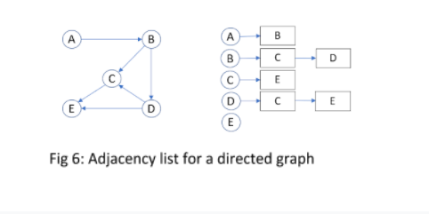
Note that the list corresponding to node E is empty while lists corresponding to nodes B and D have 2 entries each.

Similarly, adjacency lists for an undirected graph can also be constructed. Fig 7 provides an example of an undirected graph along with its adjacency list for better understanding. 

Adjacency list enables faster search process in comparison to adjacency matrix. However, it is not the best representation of graphs especially when it comes to adding or removing nodes. For example, deleting a node would involve looking through all the adjacency lists to remove a particular node from all lists. 

Tirthankar Pal

MBA from IIT Kharagpur with GATE, GMAT, IIT Kharagpur Written Test, and Interview

2 year PGDM (E-Business) from Welingkar, Mumbai

4 years of Bachelor of Science (Hons) in Computer Science from the National Institute of Electronics and Information Technology

Google and Hubspot Certification

Brain Bench Certification in C++, VC++, Data Structure and Project Management

10 years of Experience in Software Development out of that 6 years 8 months in Wipro

Selected in Six World Class UK Universities:-

King's College London, Durham University, University of Exeter, University of Sheffield, University of Newcastle, University of Leeds

Data Structures and Algorithms (Merge Sort) - Tirthankar Pal - MBA from IIT Kharagpur, GATE, GMAT, IIT Written Test, Interview were a part of MBA Entrance, B.S. in Computer Science from NIELIT

Merge sort is a sorting technique based on divide and conquer technique. With worst-case time complexity being Ο(n log n), it is one of the most respected algorithms.

Merge sort first divides the array into equal halves and then combines them in a sorted manner.

How Merge Sort Works?

To understand merge sort, we take an unsorted array as the following −

We know that merge sort first divides the whole array iteratively into equal halves unless the atomic values are achieved. We see here that an array of 8 items is divided into two arrays of size 4.

This does not change the sequence of appearance of items in the original. Now we divide these two arrays into halves.

We further divide these arrays and we achieve atomic value which can no more be divided.

Now, we combine them in exactly the same manner as they were broken down. Please note the color codes given to these lists.

We first compare the element for each list and then combine them into another list in a sorted manner. We see that 14 and 33 are in sorted positions. We compare 27 and 10 and in the target list of 2 values we put 10 first, followed by 27. We change the order of 19 and 35 whereas 42 and 44 are placed sequentially.

In the next iteration of the combining phase, we compare lists of two data values, and merge them into a list of found data values placing all in a sorted order.

After the final merging, the list should look like this −

Now we should learn some programming aspects of merge sorting.

Algorithm

Merge sort keeps on dividing the list into equal halves until it can no more be divided. By definition, if it is only one element in the list, it is sorted. Then, merge sort combines the smaller sorted lists keeping the new list sorted too.

Step 1 − if it is only one element in the list it is already sorted, return.
Step 2 − divide the list recursively into two halves until it can no more be divided.
Step 3 − merge the smaller lists into new list in sorted order.

Pseudocode

We shall now see the pseudocodes for merge sort functions. As our algorithms point out two main functions − divide & merge.

Merge sort works with recursion and we shall see our implementation in the same way.

procedure mergesort( var a as array )
   if ( n == 1 ) return a

   var l1 as array = a[0] ... a[n/2]
   var l2 as array = a[n/2+1] ... a[n]

   l1 = mergesort( l1 )
   l2 = mergesort( l2 )

   return merge( l1, l2 )
end procedure

procedure merge( var a as array, var b as array )

   var c as array
   while ( a and b have elements )
      if ( a[0] > b[0] )
         add b[0] to the end of c
         remove b[0] from b
      else
         add a[0] to the end of c
         remove a[0] from a
      end if
   end while
   
   while ( a has elements )
      add a[0] to the end of c
      remove a[0] from a
   end while
   
   while ( b has elements )
      add b[0] to the end of c
      remove b[0] from b
   end while
   
   return c
	
end 

Tirthankar Pal
MBA from IIT Kharagpur with GATE, GMAT, IIT Kharagpur Written Test, and Interview
2 year PGDM (E-Business) from Welingkar, Mumbai
4 years of Bachelor of Science (Hons) in Computer Science from the National Institute of Electronics and Information Technology
Google and Hubspot Certification
Brain Bench Certification in C++, VC++, Data Structure and Project Management
10 years of Experience in Software Development out of that 6 years 8 months in Wipro
Selected in Six World Class UK Universities:-
King's College London, Durham University, University of Exeter, University of Sheffield, University of Newcastle, University of Leeds

Data Structures and Algorithms (Binary Search Tree, Insertion Sort and Bubble Sort) - Tirthankar Pal - MBA from IIT Kharagpur, GATE, GMAT, IIT Written Test, Interview were a part of MBA Entrance, B.S. in Computer Science from NIELIT

 

Algorithm For Binary Search

In the binary search method, the collection is repeatedly divided into half and the key element is searched in the left or right half of the collection depending on whether the key is less than or greater than the mid element of the collection.

A simple Binary Search Algorithm is as follows:

1. Calculate the mid element of the collection.
2. Compare the key items with the mid element.
3. If key = middle element, then we return the mid index position for the key found.
4. Else If key > mid element, then the key lies in the right half of the collection. Thus repeat steps 1 to 3 on the lower (right) half of the collection.
5. Else key < mid element, then the key is in the upper half of the collection. Hence you need to repeat the binary search in the upper half.

As you can see from the above steps, in Binary search, half the elements in the collection are ignored just after the first comparison.

Note that the same sequence of steps holds for iterative as well as recursive binary search.

Let’s illustrate the binary search algorithm using an example.

For example, take the following sorted array of 10 elements.

Let’s calculate the middle location of the array.

Mid = 0+9/2 = 4

#1) Key = 21

First, we will compare the key value with the [mid] element and we find that the element value at mid = 21.

Thus we find that key = [mid]. Hence the key is found at position 4 in the array.

#2) Key = 25

We first compare the key value to mid. As (21 < 25), we will directly search for the key in the upper half of the array.

Now again we will find the mid for the upper half of the array.

Mid = 4+9/2 = 6

The value at location [mid] = 25

Now we compare the key element with the mid element. So (25 == 25), hence we have found the key at location [mid] = 6.

Thus we repeatedly divide the array and by comparing the key element with the mid, we decide in which half to search for the key. Binary search is more efficient in terms of time and correctness and is a lot faster too.

Insertion Sort Algorithm

To sort an array of size N in ascending order: 

• Iterate from arr[1] to arr[N] over the array. 
• Compare the current element (key) to its predecessor. 
• If the key element is smaller than its predecessor, compare it to the elements before. Move the greater elements one position up to make space for the swapped element.

Bubble Sort Algorithm

• Run a nested for loop to traverse the input array using two variables i and j, such that 0 ≤ i < n-1 and 0 ≤ j < n-i-1
• If arr[j] is greater than arr[j+1] then swap these adjacent elements, else move on
• Print the sorted array

Tirthankar Pal

MBA from IIT Kharagpur with GATE, GMAT, IIT Kharagpur Written Test, and Interview

2 year PGDM (E-Business) from Welingkar, Mumbai

4 years of Bachelor of Science (Hons) in Computer Science from the National Institute of Electronics and Information Technology

Google and Hubspot Certification

Brain Bench Certification in C++, VC++, Data Structure and Project Management

10 years of Experience in Software Development out of that 6 years 8 months in Wipro

Selected in Six World Class UK Universities:-

King's College London, Durham University, University of Exeter, University of Sheffield, University of Newcastle, University of Leeds

• 
  
  

Data Structures and Algorithms (Binary Search Tree) - Tirthankar Pal - MBA from IIT Kharagpur, GATE, GMAT, IIT Written Test, Interview were a part of MBA Entrance, B.S. in Computer Science from NIELIT

Trees and Binary Search Tree

A tree is a data structure composed of nodes that has the following characteristics:

1.      Each tree has a root node (at the top) having some value.

2.      The root node has zero or more child nodes.

3.      Each child node has zero or more child nodes, and so on. This create a subtree in the tree. Every node has it’s own subtree made up of his children and their children, etc. This means that every node on its own can be a tree.

A binary search tree (BST) adds these two characteristics:

1.      Each node has a maximum of up to two children.

2.      For each node, the values of its left descendent nodes are less than that of the current node, which in turn is less than the right descendent nodes (if any).

struct node* search(int data){

               struct node *current = root;

                 printf("Visiting elements: ");

   while(current->data != data){

                               if(current != NULL) {

                     printf("%d ",current->data);

                     //go to left tree

              if(current->data > data){

                          current = current->leftChild;

              }//else go to right tree

                    else {                

                  current = current->rightChild;

         }

            //not found

           if(current == NULL){

            return NULL;

         }

      }                                          

   }

   return current;

}

Tirthankar Pal
MBA from IIT Kharagpur with GATE, GMAT, IIT Kharagpur Written Test, and Interview
2 year PGDM (E-Business) from Welingkar, Mumbai
4 years of Bachelor of Science (Hons) in Computer Science from the National Institute of Electronics and Information Technology
Google and Hubspot Certification
Brain Bench Certification in C++, VC++, Data Structure and Project Management
10 years of Experience in Software Development out of that 6 years 8 months in Wipro
Selected in Six World Class UK Universities:-
King's College London, Durham University, University of Exeter, University of Sheffield, University of Newcastle, University of Leeds