Wednesday, September 28, 2022

Data Structures and Algorithms (Heap Sort) - Tirthankar Pal - MBA from IIT Kharagpur, GATE, GMAT, IIT Written Test, Interview were a part of MBA Entrance, B.S. in Computer Science from NIELIT

Heap Sort Algorithm

In this tutorial, you will learn about the heap sort algorithm and its implementation in Python, Java, C, and C++.

Heap Sort is a popular and efficient sorting algorithm in computer programming. Learning how to write the heap sort algorithm requires knowledge of two types of data structures - arrays and trees.

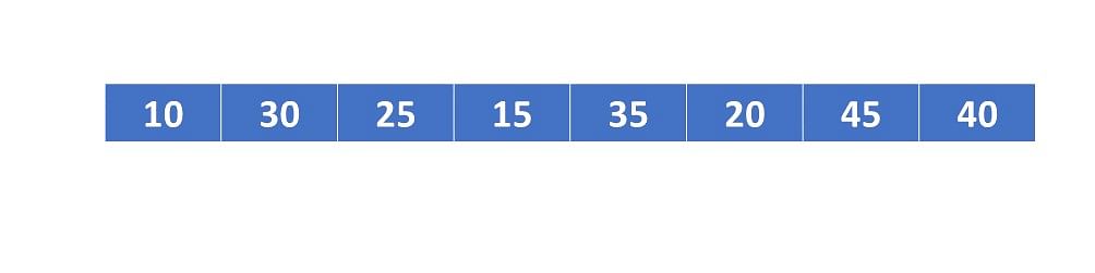
The initial set of numbers that we want to sort is stored in an array e.g. [10, 3, 76, 34, 23, 32] and after sorting, we get a sorted array [3,10,23,32,34,76].

Heap sort works by visualizing the elements of the array as a special kind of complete binary tree called a heap.

Note: As a prerequisite, you must know about a complete binary tree and heap data structure.


Relationship between Array Indexes and Tree Elements

A complete binary tree has an interesting property that we can use to find the children and parents of any node.

If the index of any element in the array is i, the element in the index 2i+1 will become the left child and element in 2i+2 index will become the right child. Also, the parent of any element at index i is given by the lower bound of (i-1)/2.

on the left, there is a graph and on the right there is an array representation of the same graph to compare equivalent indices
Relationship between array and heap indices

Let's test it out,

Left child of 1 (index 0)
= element in (2*0+1) index 
= element in 1 index 
= 12


Right child of 1
= element in (2*0+2) index
= element in 2 index 
= 9

Similarly,
Left child of 12 (index 1)
= element in (2*1+1) index
= element in 3 index
= 5

Right child of 12
= element in (2*1+2) index
= element in 4 index
= 6

Let us also confirm that the rules hold for finding parent of any node

Parent of 9 (position 2) 
= (2-1)/2 
= ½ 
= 0.5
~ 0 index 
= 1

Parent of 12 (position 1) 
= (1-1)/2 
= 0 index 
= 1

Understanding this mapping of array indexes to tree positions is critical to understanding how the Heap Data Structure works and how it is used to implement Heap Sort.


What is Heap Data Structure?

Heap is a special tree-based data structure. A binary tree is said to follow a heap data structure if

  • it is a complete binary tree
  • All nodes in the tree follow the property that they are greater than their children i.e. the largest element is at the root and both its children and smaller than the root and so on. Such a heap is called a max-heap. If instead, all nodes are smaller than their children, it is called a min-heap

The following example diagram shows Max-Heap and Min-Heap.

max heap min heap comparison
Max Heap and Min Heap

To learn more about it, please visit Heap Data Structure.


How to "heapify" a tree

Starting from a complete binary tree, we can modify it to become a Max-Heap by running a function called heapify on all the non-leaf elements of the heap.

Since heapify uses recursion, it can be difficult to grasp. So let's first think about how you would heapify a tree with just three elements.

heapify(array)
    Root = array[0]
    Largest = largest( array[0] , array [2*0 + 1]. array[2*0+2])
    if(Root != Largest)
          Swap(Root, Largest)
graph shows how base case of heapify works
Heapify base cases

The example above shows two scenarios - one in which the root is the largest element and we don't need to do anything. And another in which the root had a larger element as a child and we needed to swap to maintain max-heap property.

If you're worked with recursive algorithms before, you've probably identified that this must be the base case.

Now let's think of another scenario in which there is more than one level.

image showing tree data with root element containing two max-heap subtrees
How to heapify root element when its subtrees are already max heaps

The top element isn't a max-heap but all the sub-trees are max-heaps.

To maintain the max-heap property for the entire tree, we will have to keep pushing 2 downwards until it reaches its correct position.

steps to heapify root element when both of its subtrees are already max-heaps
How to heapify root element when its subtrees are max-heaps

Thus, to maintain the max-heap property in a tree where both sub-trees are max-heaps, we need to run heapify on the root element repeatedly until it is larger than its children or it becomes a leaf node.

void heapify(int arr[], int n, int i) {
  // Find largest among root, left child and right child
  int largest = i;
  int left = 2 * i + 1;
  int right = 2 * i + 2;

  if (left < n && arr[left] > arr[largest])
    largest = left;

  if (right < n && arr[right] > arr[largest])
    largest = right;

    // Swap and continue heapifying if root is not largest
    if (largest != i) {
      swap(&arr[i], &arr[largest]);
      heapify(arr, n, largest);
  }
}

This function works for both the base case and for a tree of any size. We can thus move the root element to the correct position to maintain the max-heap status for any tree size as long as the sub-trees are max-heaps.


Build max-heap

To build a max-heap from any tree, we can thus start heapifying each sub-tree from the bottom up and end up with a max-heap after the function is applied to all the elements including the root element.

In the case of a complete tree, the first index of a non-leaf node is given by n/2 - 1. All other nodes after that are leaf-nodes and thus don't need to be heapified.

So, we can build a maximum heap as

    // Build heap (rearrange array)
    for (int i = n / 2 - 1; i >= 0; i--)
      heapify(arr, n, i);
steps to build max heap for heap sort
Create array and calculate i
steps to build max heap for heap sort
Steps to build max heap for heap sort
steps to build max heap for heap sort
Steps to build max heap for heap sort
steps to build max heap for heap sort
Steps to build max heap for heap sort

As shown in the above diagram, we start by heapifying the lowest smallest trees and gradually move up until we reach the root element.

If you've understood everything till here, congratulations, you are on your way to mastering the Heap sort.


Working of Heap Sort

  1. Since the tree satisfies Max-Heap property, then the largest item is stored at the root node.
  2. Swap: Remove the root element and put at the end of the array (nth position) Put the last item of the tree (heap) at the vacant place.
  3. Remove: Reduce the size of the heap by 1.
  4. Heapify: Heapify the root element again so that we have the highest element at root.
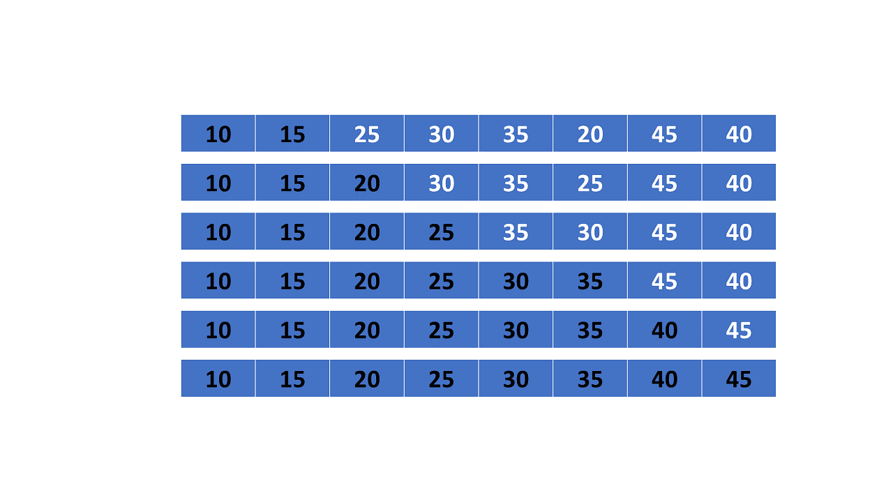
  5. The process is repeated until all the items of the list are sorted.
procedures for implementing heap sort
Swap, Remove, and Heapify

The code below shows the operation.

    // Heap sort
    for (int i = n - 1; i >= 0; i--) {
      swap(&arr[0], &arr[i]);

      // Heapify root element to get highest element at root again
      heapify(arr, i, 0);
    }

Heap Sort Code in Python, Java, and C/C++

# Heap Sort in python


  def heapify(arr, n, i):
      # Find largest among root and children
      largest = i
      l = 2 * i + 1
      r = 2 * i + 2
  
      if l < n and arr[i] < arr[l]:
          largest = l
  
      if r < n and arr[largest] < arr[r]:
          largest = r
  
      # If root is not largest, swap with largest and continue heapifying
      if largest != i:
          arr[i], arr[largest] = arr[largest], arr[i]
          heapify(arr, n, largest)
  
  
  def heapSort(arr):
      n = len(arr)
  
      # Build max heap
      for i in range(n//2, -1, -1):
          heapify(arr, n, i)
  
      for i in range(n-1, 0, -1):
          # Swap
          arr[i], arr[0] = arr[0], arr[i]
  
          # Heapify root element
          heapify(arr, i, 0)
  
  
  arr = [1, 12, 9, 5, 6, 10]
  heapSort(arr)
  n = len(arr)
  print("Sorted array is")
  for i in range(n):
      print("%d " % arr[i], end='')
  

Heap Sort Complexity

Time Complexity 
BestO(nlog n)
WorstO(nlog n)
AverageO(nlog n)
Space ComplexityO(1)
StabilityNo

Heap Sort has O(nlog n) time complexities for all the cases ( best case, average case, and worst case).

Let us understand the reason why. The height of a complete binary tree containing n elements is log n

As we have seen earlier, to fully heapify an element whose subtrees are already max-heaps, we need to keep comparing the element with its left and right children and pushing it downwards until it reaches a point where both its children are smaller than it.

In the worst case scenario, we will need to move an element from the root to the leaf node making a multiple of log(n) comparisons and swaps.

During the build_max_heap stage, we do that for n/2 elements so the worst case complexity of the build_heap step is n/2*log n ~ nlog n.

During the sorting step, we exchange the root element with the last element and heapify the root element. For each element, this again takes log n worst time because we might have to bring the element all the way from the root to the leaf. Since we repeat this n times, the heap_sort step is also nlog n.

Also since the build_max_heap and heap_sort steps are executed one after another, the algorithmic complexity is not multiplied and it remains in the order of nlog n.

Also it performs sorting in O(1) space complexity. Compared with Quick Sort, it has a better worst case ( O(nlog n) ). Quick Sort has complexity O(n^2) for worst case. But in other cases, Quick Sort is fast. Introsort is an alternative to heapsort that combines quicksort and heapsort to retain advantages of both: worst case speed of heapsort and average speed of quicksort.


Heap Sort Applications

Systems concerned with security and embedded systems such as Linux Kernel use Heap Sort because of the O(n log n) upper bound on Heapsort's running time and constant O(1) upper bound on its auxiliary storage.

Although Heap Sort has O(n log n) time complexity even for the worst case, it doesn't have more applications ( compared to other sorting algorithms like Quick Sort, Merge Sort ). However, its underlying data structure, heap, can be efficiently used if we want to extract the smallest (or largest) from the list of items without the overhead of keeping the remaining items in the sorted order. For e.g Priority Queues.

Tirthankar Pal

MBA from IIT Kharagpur with GATE, GMAT, IIT Kharagpur Written Test, and Interview

2 year PGDM (E-Business) from Welingkar, Mumbai

4 years of Bachelor of Science (Hons) in Computer Science from the National Institute of Electronics and Information Technology

Google and Hubspot Certification

Brain Bench Certification in C++, VC++, Data Structure and Project Management

10 years of Experience in Software Development out of that 6 years 8 months in Wipro

Selected in Six World Class UK Universities:-

King's College London, Durham University, University of Exeter, University of Sheffield, University of Newcastle, University of Leeds


Data Structures and Algorithms (DFS in a graph) - Tirthankar Pal - MBA from IIT Kharagpur, GATE, GMAT, IIT Written Test, Interview were a part of MBA Entrance, B.S. in Computer Science from NIELIT

DFS in a graph.

Depth-first search (DFS) is an algorithm for traversing or searching tree or graph data structures. The algorithm starts at the root node (selecting some arbitrary node as the root node in the case of a graph) and explores as far as possible along each branch before backtracking. Extra memory, usually a stack, is needed to keep track of the nodes discovered so far along a specified branch which helps in backtracking of the graph.

A version of depth-first search was investigated in the 19th century by French mathematician Charles Pierre Trémaux[1] as a strategy for solving mazes

Properties[edit]

The time and space analysis of DFS differs according to its application area. In theoretical computer science, DFS is typically used to traverse an entire graph, and takes time ,[4] where  is the number of vertices and  the number of edges. This is linear in the size of the graph. In these applications it also uses space  in the worst case to store the stack of vertices on the current search path as well as the set of already-visited vertices. Thus, in this setting, the time and space bounds are the same as for breadth-first search and the choice of which of these two algorithms to use depends less on their complexity and more on the different properties of the vertex orderings the two algorithms produce.

For applications of DFS in relation to specific domains, such as searching for solutions in artificial intelligence or web-crawling, the graph to be traversed is often either too large to visit in its entirety or infinite (DFS may suffer from non-termination). In such cases, search is only performed to a limited depth; due to limited resources, such as memory or disk space, one typically does not use data structures to keep track of the set of all previously visited vertices. When search is performed to a limited depth, the time is still linear in terms of the number of expanded vertices and edges (although this number is not the same as the size of the entire graph because some vertices may be searched more than once and others not at all) but the space complexity of this variant of DFS is only proportional to the depth limit, and as a result, is much smaller than the space needed for searching to the same depth using breadth-first search. For such applications, DFS also lends itself much better to heuristic methods for choosing a likely-looking branch. When an appropriate depth limit is not known a priori, iterative deepening depth-first search applies DFS repeatedly with a sequence of increasing limits. In the artificial intelligence mode of analysis, with a branching factor greater than one, iterative deepening increases the running time by only a constant factor over the case in which the correct depth limit is known due to the geometric growth of the number of nodes per level.

DFS may also be used to collect a sample of graph nodes. However, incomplete DFS, similarly to incomplete BFS, is biased towards nodes of high degree.


Example[edit]

Animated example of a depth-first search

For the following graph:

An undirected graph with edges AB, BD, BF, FE, AC, CG, AE

a depth-first search starting at the node A, assuming that the left edges in the shown graph are chosen before right edges, and assuming the search remembers previously visited nodes and will not repeat them (since this is a small graph), will visit the nodes in the following order: A, B, D, F, E, C, G. The edges traversed in this search form a Trémaux tree, a structure with important applications in graph theory. Performing the same search without remembering previously visited nodes results in visiting the nodes in the order A, B, D, F, E, A, B, D, F, E, etc. forever, caught in the A, B, D, F, E cycle and never reaching C or G.

Iterative deepening is one technique to avoid this infinite loop and would reach all nodes.

Output of a depth-first search[edit]

The four types of edges defined by a spanning tree

The result of a depth-first search of a graph can be conveniently described in terms of a spanning tree of the vertices reached during the search. Based on this spanning tree, the edges of the original graph can be divided into three classes: forward edges, which point from a node of the tree to one of its descendants, back edges, which point from a node to one of its ancestors, and cross edges, which do neither. Sometimes tree edges, edges which belong to the spanning tree itself, are classified separately from forward edges. If the original graph is undirected then all of its edges are tree edges or back edges.

Vertex orderings[edit]

It is also possible to use depth-first search to linearly order the vertices of a graph or tree. There are four possible ways of doing this:

  • preordering is a list of the vertices in the order that they were first visited by the depth-first search algorithm. This is a compact and natural way of describing the progress of the search, as was done earlier in this article. A preordering of an expression tree is the expression in Polish notation.
  • postordering is a list of the vertices in the order that they were last visited by the algorithm. A postordering of an expression tree is the expression in reverse Polish notation.
  • reverse preordering is the reverse of a preordering, i.e. a list of the vertices in the opposite order of their first visit. Reverse preordering is not the same as postordering.
  • reverse postordering is the reverse of a postordering, i.e. a list of the vertices in the opposite order of their last visit. Reverse postordering is not the same as preordering.

For binary trees there is additionally in-ordering and reverse in-ordering.

For example, when searching the directed graph below beginning at node A, the sequence of traversals is either A B D B A C A or A C D C A B A (choosing to first visit B or C from A is up to the algorithm). Note that repeat visits in the form of backtracking to a node, to check if it has still unvisited neighbors, are included here (even if it is found to have none). Thus the possible preorderings are A B D C and A C D B, while the possible postorderings are D B C A and D C B A, and the possible reverse postorderings are A C B D and A B C D.

A directed graph with edges AB, BD, AC, CD

Reverse postordering produces a topological sorting of any directed acyclic graph. This ordering is also useful in control-flow analysis as it often represents a natural linearization of the control flows. The graph above might represent the flow of control in the code fragment below, and it is natural to consider this code in the order A B C D or A C B D but not natural to use the order A B D C or A C D B.

if (A) then {
    B
} else {
    C
}
D

Pseudocode[edit]

InputOutput: A recursive implementation of DFS:[5]

procedure DFS(G, v) is
    label v as discovered
    for all directed edges from v to w that are in G.adjacentEdges(v) do
        if vertex w is not labeled as discovered then
            recursively call DFS(G, w)

A non-recursive implementation of DFS with worst-case space complexity , with the possibility of duplicate vertices on the stack:[6]

procedure DFS_iterative(G, v) is
    let S be a stack
    S.push(v)
    while S is not empty do
        v = S.pop()
        if v is not labeled as discovered then
            label v as discovered
            for all edges from v to w in G.adjacentEdges(v) do 
                S.push(w)
An undirected graph with edges AB, BD, BF, FE, AC, CG, AE

These two variations of DFS visit the neighbors of each vertex in the opposite order from each other: the first neighbor of v visited by the recursive variation is the first one in the list of adjacent edges, while in the iterative variation the first visited neighbor is the last one in the list of adjacent edges. The recursive implementation will visit the nodes from the example graph in the following order: A, B, D, F, E, C, G. The non-recursive implementation will visit the nodes as: A, E, F, B, D, C, G.

The non-recursive implementation is similar to breadth-first search but differs from it in two ways:

  1. it uses a stack instead of a queue, and
  2. it delays checking whether a vertex has been discovered until the vertex is popped from the stack rather than making this check before adding the vertex.

If G is a tree, replacing the queue of the breadth-first search algorithm with a stack will yield a depth-first search algorithm. For general graphs, replacing the stack of the iterative depth-first search implementation with a queue would also produce a breadth-first search algorithm, although a somewhat nonstandard one.[7]

Another possible implementation of iterative depth-first search uses a stack of iterators of the list of neighbors of a node, instead of a stack of nodes. This yields the same traversal as recursive DFS.[8]

procedure DFS_iterative(G, v) is
    let S be a stack
    S.push(iterator of G.adjacentEdges(v))
    while S is not empty do
        if S.peek().hasNext() then
            w = S.peek().next()
            if w is not labeled as discovered then
                label w as discovered
                S.push(iterator of G.adjacentEdges(w))
        else
            S.pop()

Applications[edit]

1:01
Randomized algorithm similar to depth-first search used in generating a maze.

Algorithms that use depth-first search as a building block include:

Complexity[edit]

The computational complexity of DFS was investigated by John Reif. More precisely, given a graph , let  be the ordering computed by the standard recursive DFS algorithm. This ordering is called the lexicographic depth-first search ordering. John Reif considered the complexity of computing the lexicographic depth-first search ordering, given a graph and a source. A decision version of the problem (testing whether some vertex u occurs before some vertex v in this order) is P-complete,[12] meaning that it is "a nightmare for parallel processing".[13]: 189 

A depth-first search ordering (not necessarily the lexicographic one), can be computed by a randomized parallel algorithm in the complexity class RNC.[14] As of 1997, it remained unknown whether a depth-first traversal could be constructed by a deterministic parallel algorithm, in the complexity class NC.[15] 

Tirthankar Pal

MBA from IIT Kharagpur with GATE, GMAT, IIT Kharagpur Written Test, and Interview

2 year PGDM (E-Business) from Welingkar, Mumbai

4 years of Bachelor of Science (Hons) in Computer Science from the National Institute of Electronics and Information Technology

Google and Hubspot Certification

Brain Bench Certification in C++, VC++, Data Structure and Project Management

10 years of Experience in Software Development out of that 6 years 8 months in Wipro

Selected in Six World Class UK Universities:-

King's College London, Durham University, University of Exeter, University of Sheffield, University of Newcastle, University of Leeds


Data Structures and Algorithms (Selection Sort Algorithm) - Tirthankar Pal - MBA from IIT Kharagpur, GATE, GMAT, IIT Written Test, Interview were a part of MBA Entrance, B.S. in Computer Science from NIELIT

Write an algorithm to perform selection sort in an array.

The selection sort algorithm is a simple, yet effective sorting algorithm. A selection-based sorting algorithm is described as an in-place comparison-based algorithm that divides the list into two parts, the sorted part on the left and the unsorted part on the right. Initially, the sorted section is empty, and the unsorted section contains the entire list. When sorting a small list, selection sort can be used. 

In the selection sort, the cost of swapping is irrelevant, and all elements must be checked. The cost of writing to memory matters in selection sort, just as it does in flash memory (the number of writes/swaps is O(n) as opposed to O(n2) in bubble sort).

What Is a Selection Sort Algorithm?

  • Selection sort is an effective and efficient sort algorithm based on comparison operations.
  • It adds one element in each iteration.
  • You need to select the smallest element in the array and move it to the beginning of the array by swapping with the front element.
  • You can also accomplish this by selecting the most potent element and positioning it at the back end.
  • In each iteration, selection sort selects an element and places it in the appropriate position.

what-is-selection-sort.

Following the definition of the selection sort algorithm, you will now go over the working procedure of the selection sort algorithm in this tutorial.

Post Graduate Program: Full Stack Web Development

in Collaboration with Caltech CTMEENROLL NOW
Post Graduate Program: Full Stack Web Development

How Does the Selection Sort Algorithm Work?

Selection sort works by taking the smallest element in an unsorted array and bringing it to the front. You’ll go through each item (from left to right) until you find the smallest one. The first item in the array is now sorted, while the rest of the array is unsorted.

  • As an example, consider the array depicted below.

working-of-selection-sort-algorithm.

  • The entire list is scanned sequentially for the first position in the sorted list. You search the whole list and find that 10 is the lowest value in the first position, where 15 is stored.

working-of-selection-sort-algorithm1.

  • As a result, you replaced 15 with 10. After one iteration, the number 10, which happens to be the lowest value on the list, appears at the top of the sorted list.

working-of-selection-sort2

  • You must begin by scanning the rest of the list linearly for the second position, where 30 is located.

working-of-selection-sort-algorithm4

  • You discovered that 15 is the second lowest value on the list and should be placed second. You must switch these values.

working-of-selection-sort-algorithm5.j

  • After two iterations, the two least values are positioned at the beginning in a sorted manner.

working-of-selection-sort-algorithm6.

The same procedure is followed for the remaining array items.

The following is a visual representation of the entire sorting process.

working-of-selection-sort-final

Moving forward in this tutorial, you will see an algorithm and its pseudocode after understanding the working procedure of a selection sort algorithm.


Algorithm of the Selection Sort Algorithm

The selection sort algorithm is as follows:

Step 1: Set Min to location 0 in Step 1.

Step 2: Look for the smallest element on the list.

Step 3: Replace the value at location Min with a different value.

Step 4: Increase Min to point to the next element

Step 5: Continue until the list is sorted.

Pseudocode of Selection Sort Algorithm

The selection sort pseudocode is as follows:

function selection sort 

   array : array of items

   size : size of list

   for i = 1 to size - 1                                       

      minimum = i // set current element as minimum

      for j = i+1 to n // check the element to be minimum

         if array[j] < array[minimum] then

            minimum = j;

         end if

      end for

      if indexofMinimum != i then //swap the minimum element with the current element

         swap array[minimum] and array[i]

      end if

   end for

end function


You will now look at the performance of the selection sort algorithm in this tutorial.

The Complexity of Selection Sort Algorithm

The time complexity of the selection sort algorithm is:

  • The selection sort algorithm is made up of two nested loops.
  • It has an O (n2) time complexity due to the two nested loops.

Best Case Complexity occurs when there is no need for sorting, i.e., the array has already been sorted. The time complexity of selection sort in the best-case scenario is O. (n2).

Average Case Complexity occurs when the array elements are arranged in a jumbled order that is neither ascending nor descending correctly. The selection sort has an average case time complexity of O. (n2).

Worst-case complexity - Worst case occurs when array elements must be sorted in reverse order. Assume you need to sort the array elements in ascending order, but they are in descending order. Selection sort has a worst-case time complexity of O. (n2).

The space complexity of the selection sort algorithm is:

  • An in-place algorithm is a selection sort algorithm.
  • It performs all computations in the original array and does not use any other arrays.
  • As a result, the space complexity is O. (1).

You will now look at some applications of the selection sort algorithm in this tutorial.

Applications of Selection Sort Algorithm

The following are some applications of how to use selection sort:

  • Selection sort consistently outperforms bubble and gnome sort.
  • When memory writing is a costly operation, this can be useful.
  • In terms of the number of writes ((n) swaps versus O(n2) swaps), selection sort is preferable to insertion sort.
  • It almost always far outnumbers the number of writes made by cycle sort, even though cycle sort is theoretically optimal in terms of the number of writes.
  • This is important if writes are significantly more expensive than reads, as with EEPROM or Flash memory, where each write reduces the memory's lifespan.

Following an understanding of some applications of the selection sort algorithm, you will now look at code

Code implementation of selection sort:

#include <stdio.h>  

#include <conio.h>

#include <stdlib.h>

void selection(int array[], int n)  

{  

    int i, j, minimum;  

    for (i = 0; i < n-1; i++) //Move one at a time unsorted subarray boundary

    {  

        minimum = i; //in an unsorted array, the minimum element         

        for (j = i+1; j < n; j++)  

        if (array[j] < array[minimum])  

            minimum = j;  

    int temp = array[minimum]; // Replace the first element with the minimum element.

    array[minimum] = array[i];  

    array[i] = temp;  

    }  

}  

void printArr(int array1[], int n) //function to print the array//

{  

    int i;  

    for (i = 0; i < n; i++)  

        printf("%d ", array1[i]);  

}  

int main()  

{  

    int array1[] = { 15, 30, 29, 14, 39, 11 };  

    int n = sizeof(array1) / sizeof(array1[0]);  

    printf(" An array before sorting: - \n");  

    printArr(array1, n);  

    selection(array1, n);  

    printf("\nAn Array after sorting- \n");    

    printArr(array1, n);  

    return 0;  

}  

Output

output-of-selection-sort-algorithm

Tirthankar Pal

MBA from IIT Kharagpur with GATE, GMAT, IIT Kharagpur Written Test, and Interview

2 year PGDM (E-Business) from Welingkar, Mumbai

4 years of Bachelor of Science (Hons) in Computer Science from the National Institute of Electronics and Information Technology

Google and Hubspot Certification

Brain Bench Certification in C++, VC++, Data Structure and Project Management

10 years of Experience in Software Development out of that 6 years 8 months in Wipro

Selected in Six World Class UK Universities:-

King's College London, Durham University, University of Exeter, University of Sheffield, University of Newcastle, University of Leeds